The previous articles talked about the CNN CNN, but it may not be very clear about the features it extracts at each layer and the training process, so this section is mainly through the visualization of the model. The neural network is in each layer. How to train. We know that the neural network itself contains a series of feature extractors. The ideal feature map should be sparse and contain typical local information. Visualizing the model can have some intuitive knowledge and help us to debug the model. For example, the feature map is close to the original image, indicating that it has not learned any features; or it is almost a solid-colored map, indicating that it is too sparse. It may be We have too many feature maps (too many feature_maps also reflect that the convolution kernel is too small). There are many kinds of visualization, such as: feature map visualization, weight visualization, etc. I use the feature map visualization as an example.
Model visualization
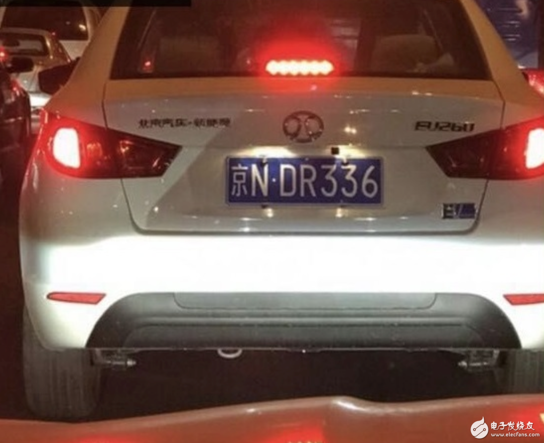
Because I did not search for googLeNet incepTIon v3 which was pre-trained on the imagenet 1000 classified dataset using paddlepaddle, so I used keras to do the experiment. The following diagram is used as input:
Enter picture
Beiqi Saab D50:

Feature map visualization
Take the first 15 layers of the network and take the first 3 feature maps for each layer.
Beiqi Saab D50 feature map:

Looking from left to right, you can see the entire feature extraction process, some separate backgrounds, some extracted outlines, and some extracted color differences, but you can also find that the middle two feature maps in the 10th and 11th layers are solid colors. The number of layer feature maps is a little bit more. In addition, the halo of Beiqi Saab D50 has more obvious effect on the halo effect in feature map.
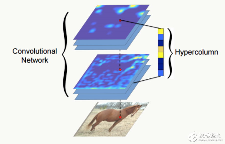
Hypercolumns Usually we represent the last full-connection layer of a neural network as a feature of the entire picture, but this representation may be too coarse (as can be seen from the above feature map visualization), and it is impossible to accurately describe features in the local space. The first layer of spatial characteristics of the network is too precise and lacks semantic information (such as color differences, contours, etc.). Therefore, the paper “Hypercolumns for Object Segmenta TIon and Fine-grained Localiza- tion†has proposed a new feature representation method: Hypercolumns— Defining a pixel's hypercolumn as a vector of all the active output values ​​of the cnn unit corresponding to the pixel's position). The tradeoff is better than the previous two problems.

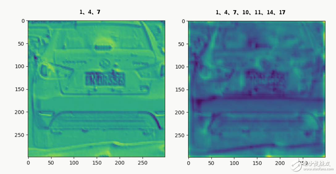
The feature maps of the 1st, 4th, and 7th floors of Beiqi Shenbao D50's 1st, 4th, and 7th levels, and the 1, 4, 7, 10, 11, 14, 17th floor feature maps are averaged and visualized as follows:

Code practice
# -*- coding: utf-8 -*-
From keras.applicaTIons import InceptionV3
From keras.applications.inception_v3 import preprocess_input
From keras.preprocessing import image
From keras.models import Model
From keras.applications.imagenet_utils import decode_predictions
Import numpy as np
Import cv2
From cv2 import *
Import matplotlib.pyplot as plt
Import scipy as sp
From scipy.misc import toimage
Def test_opencv():
# loading camera
Cam = VideoCapture(0) # 0 -> camera serial number, if there are two three four cameras, which number to call up
# Capture 5 small pictures
For x in range(0, 5):
s, img = cam.read()
If s:
Imwrite("o-" + str(x) + ".jpg", img)
Def load_original(img_path):
# Compress the original picture to 299*299 size
Im_original = cv2.resize(cv2.imread(img_path), (299, 299))
Im_converted = cv2.cvtColor(im_original, cv2.COLOR_BGR2RGB)
Plt.figure(0)
Plt.subplot(211)
Plt.imshow(im_converted)
Return im_original
Def load_fine_tune_googlenet_v3(img):
# Load fine-tuning googlenet v3 model and make predictions
Model = InceptionV3(include_top=True, weights='imagenet')
Model.summary()
x = image.img_to_array(img)
x = np.expand_dims(x, axis=0)
x = preprocess_input(x)
Preds = model.predict(x)
Print('Predicted:', decode_predictions(preds))
Plt.subplot(212)
Plt.plot(preds.ravel())
Plt.show()
Return model, x
Def extract_features(ins, layer_id, filters, layer_num):
'''
Extracts a specified number of feature maps for a given model and outputs it to a map.
:param ins: model instance
:param layer_id: Extracts the specified layer features
:param filters: number of feature maps extracted per layer
:param layer_num: how many feature maps are extracted
:return: None
'''
If len(ins) != 2:
Print('parameter error:(model, instance)')
Return None
Model = ins[0]
x = ins[1]
If type(layer_id) == type(1):
Model_extractfeatures = Model(input=model.input, output=model.get_layer(index=layer_id).output)
Else:
Model_extractfeatures = Model(input=model.input, output=model.get_layer(name=layer_id).output)
Fc2_features = model_extractfeatures.predict(x)
If filters > len(fc2_features[0][0][0]):
Print('layer number error.', len(fc2_features[0][0][0]),',',filters)
Return None
For i in range(filters):
Plt.subplots_adjust(left=0, right=1, bottom=0, top=1)
Plt.subplot(filters, layer_num, layer_id + 1 + i * layer_num)
Plt.axis("off")
If i < len(fc2_features[0][0][0]):
Plt.imshow(fc2_features[0, :, :, i])
# Number of layers, models, and convolutions
Def extract_features_batch(layer_num, model, filters):
'''
Batch extraction features
:param layer_num: number of layers
:param model: Model
:param filters: number of feature maps
:return: None
'''
Plt.figure(figsize=(filters, layer_num))
Plt.subplot(filters, layer_num, 1)
For i in range(layer_num):
Extract_features(model, i, filters, layer_num)
Plt.savefig('sample.jpg')
Plt.show()
Def extract_features_with_layers(layers_extract):
'''
Extract hypercolumn and visualize it.
:param layers_extract: Specified layer list
:return: None
'''
Hc = extract_hypercolumn(x[0], layers_extract, x[1])
Ave = np.average(hc.transpose(1, 2, 0), axis=2)
Plt.imshow(ave)
Plt.show()
Def extract_hypercolumn(model, layer_indexes, instance):
'''
Extract the hypercolumn vector of the specified layer of the specified model
:param model: Model
:param layer_indexes: layer id
:param instance: Model
:return:
'''
Feature_maps = []
For i in layer_indexes:
Feature_maps.append(Model(input=model.input, output=model.get_layer(index=i).output).predict(instance))
Hypercolumns = []
For convmap in feature_maps:
For i in convmap[0][0][0]:
Upscaled = sp.misc.imresize(convmap[0, :, :, i], size=(299, 299), mode="F", interp='bilinear')
Hypercolumns.append(upscaled)
Return np.asarray(hypercolumns)
If __name__ == '__main__':
Img_path = '~/auto1.jpg'
Img = load_original(img_path)
x = load_fine_tune_googlenet_v3(img)
Extract_features_batch(15, x, 3)
Extract_features_with_layers([1, 4, 7])
Extract_features_with_layers([1, 4, 7, 10, 11, 14, 17])
to sum up
There are also some websites that do a good job of visualizing CNN. For example, this website: http://shixialiu.com/publications/cnnvis/demo/. Everyone can use different convolution kernel sizes and numbers when training. Look at the middle course of training. PaddlePaddle also recently opened VisaulDL, a visualization tool. In the next article, we will talk about the visualDL of paddlepaddle and the tensorboard of tesorflow.
Wooden Speakers,Creative Wooden Speaker,Wooden Portable Speaker,Wooden Box Pc Speaker
Comcn Electronics Limited , https://www.comencnspeaker.com